
A step-drawdown test is a single-well test that is frequently conducted after well development to determine well efficiency and correctly size the production pump. Pumping rates are constant during steps which are of sufficient duration, about 1–4 hours, for water levels to change minimally at the end of each step (Halford and Kuniansky, 2002). Successively greater discharge rates are pumped during subsequent steps, where three to five discharge rates typically are tested. Water levels are measured prior to pumping, during each step, and during recovery so that drawdowns can be estimated.
Transmissivity and well-loss coefficients can be estimated from step drawdown data with the workbook, StepDrawdown.v4.xlsm. The 2019 workbook accounts for linear and non-linear well losses while using graphical techniques to better estimate transmissivity (Odeh and Jones, 1965). Drawdown (s) and flow-rate (Q) data are transformed by plotting drawdowns divided by flow rates (s/Qstep) against flow-weighted, dimensionless times (Figure 1).
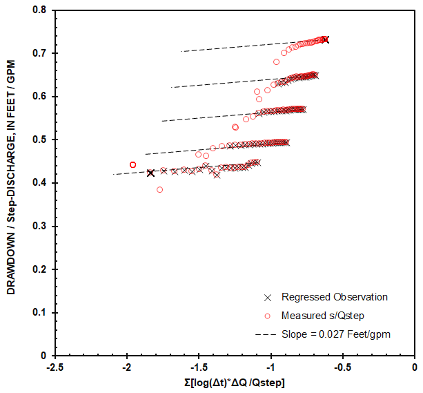
Transformed data theoretically should plot in a straight line, where transmissivity is inversely proportional to the slope (Lee, 1982). Interpretation differs from Cooper-Jacob (1946) because discharge is incorporated in the estimated slope. Transmissivity is,
T = 2.303 QCONVERT / 4 / π / Slope or 0.1832 QCONVERT / Slope, where
T is transmissivity (L²/T),
QCONVERT converts flow to consistent units, e.g. 192.5 gpm/[ft³/d], and
Slope (T/L²) estimated from flow-normalized drawdown plot.
Equation for transmissivity simplifies to,
T = 35.3 / Slope in field units of ft²/d, ft, and gpm.
Discrete steps plot separately because of non-linear, well losses. Measured s/Qstep depart from straight lines at the beginning of each step because of wellbore storage. Step drawdowns were analyzed with a flow-normalized drawdown plot in a previously developed workbook (Halford
and Kuniansky, 2002). Well-loss model and parameter estimation techniques were improved in the workbook, StepDrawdown.v4.xlsm.
Transmissivity estimates are improved with the flow-normalized drawdown plot, because effects of transmissivity on drawdowns are isolated from well-losses (Figure 1). Transmissivity can be adjusted manually to best explain late-time drawdowns during each step, while visually ignoring anomalies from unsteady flow rates and wellbore storage. These anomalies result primarily from the analytical model not simulating wellbore storage. These observations are eliminated from the regression by assigning weights of 0 to minimize their effects on estimates of well-loss coefficients . The flow-normalized drawdown plot also makes other departures between measured drawdowns and analytical model apparent such as the departure between measured and simulated slopes at highest pumping rate of 600 gpm (Figure 1, s/Qstep>0.7). Transmissivity of the aquifer likely was reduced by dewatering transmissive fractures.
The analytical model assumes that the aquifer can be described with the Theis (1935) solution and well losses have linear and non-linear components (Rorabaugh, 1953). Drawdown in the aquifer and well losses are simulated with the equation:
sW = B(t)Q(t) + B´Q + CQ², where
sW is total drawdown in the well,
B(t)Q(t) is time-dependent drawdown in aquifer,
t is the current time,
B´Q is linear well loss during a step,
CQ² is non-linear well loss during a step, and
Q is current discharge.
Drawdown in the aquifer, B(t)Q(t), is solved with superimposed Theis (1935) solutions that evaluate all pumping rates from the beginning of the step-drawdown test to the current time (t). Well losses are the summation of B´Q and CQ². This formulation differs from Rorabaugh (1953), where drawdown in the aquifer, B(t)Q(t), and linear well loss, B´Q, were combined in the term BQ.
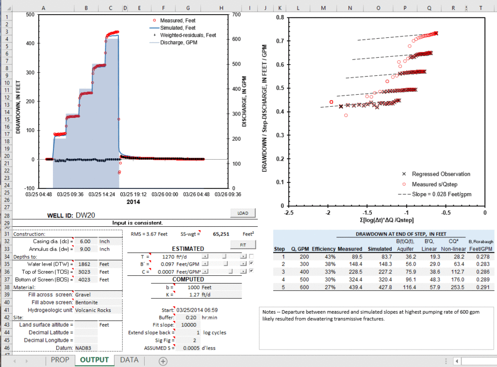
Step-drawdown data can be interpreted in the workbook, StepDrawdown.v4.xlsm to estimate transmissivity and well-loss coefficients (Figure 2). A continuous series of antecedent, pumping, and recovery water levels in the pumped well are specified as depth to water or water level above the transducer. Step discharges are specified in a table. Step-drawdowns, recoveries, and flow rates are plotted on a cartesian plot and a flow-normalized drawdown plot. Data sets are converted to drawdowns in preferred units of analysis and estimates of T, B´, and C are initialized with the “LOAD” button. Fit between straight line and plotted data can be refined visually to ignore outliers in the flow-normalized drawdown plot by estimating T with scroll bar in cell H34 on the OUTPUT page. Well-loss coefficients B´ and C can be adjusted manually with scroll bars in cells H35 and H36 or regressed with the “FIT” button in cell H32 (Figure 2). Estimated transmissivity, T, and well-loss coefficients, B´ and C, are reported in user-specified units and significant digits. Average hydraulic conductivity is reported by assuming screen length adequately approximates aquifer thickness. Well efficiency is reported at the end of each step along with measured and simulated drawdowns.
StepDrawdown.v4.xlsm and explanatory PDF can be downloaded with the following link. This workbook and other workbook applications are better used on local drives instead of a network drive. StepDrawdown.v4.xlsm workbook requires that the Solver is installed and the workbook is not opened from within a zip file. The fitting routine will stop and warn the user if the Solver is not installed. User will be warned and workbook will be closed if opened from within a zip file.
VBA macros & Trust Center
More macro functions default to being disabled through either Microsoft updates or IT departments engaging in their natural function. Please check your Trust Center settings.
Download
Revisions
May 2, 2020—Revisions in version 2 corrected an error in well loss calculations if negative (-) flow rates were specified. Well loss equation, s-well = B * dQ + C * dQ^2, incorrectly calculates negative loss for B term and positive loss for C term if dQ less than zero. Revision notes if dQ is less than 0 and correctly applies negative to B and C terms.
October 18, 2022—Revisions in version 3 include the following. Safeguards were added to check that the Solver is installed and the workbook is not opened from within a zip file.
October 5, 2025—Revisions in version 4 include the following. Maximum difference between minimum and maximum pumping rate of a step specified, which keeps chart of transformed drawdown and flow-rate useable.
Suggested Citation
Halford, Keith, 2025, Step-Drawdown–A workbook for analysis of step drawdown tests, version 4, Halford Hydrology LLC web page, accessed October 2025, at https://halfordhydrology.com/step-drawdown/
References
Cooper, H.H., and C.E. Jacob. 1946. A generalized graphical method for evaluating formation constants and summarizing well field history. American Geophysical Union Transactions 27: 526–534. https://doi.org/10.1029/TR027i004p00526
Halford, K.J. and E.L. Kuniansky 2002, Documentation of spreadsheets for the analysis of aquifer pumping and slug test data, USGS OF 02-197 https://pubs.usgs.gov/of/2002/ofr02197/
Lee, John, 1982, Well Testing: Society of Petroleum Engineers of AIME: New York, 159 p. https://www.amazon.com/Well-Testing-SPE-textbook-John/dp/0895203170
Odeh, Souad and G.L. Jones, 1965, Pressure Drawdown Analysis, Variable-Rate Case. Journal of Petroleum Technology 17. 960-964 https://www.researchgate.net/publication/240779570_Pressure_Drawdown_Analysis_Variable-Rate_Case
Rorabaugh, M.I., 1953, Graphical and theoretical analysis of step-drawdown test of artesian well: Proceedings of American Society of Civil Engineers, vol. 79, no. 362, 23 p.
Theis, C.V., 1935, The relation between the lowering of the Piezometric surface and the rate and duration of discharge of a well using ground-water Storage: Transactions of the American Geophysical Union, v. 16, no. 2, p. 519–524, https://doi.org/10.1029/TR016i002p00519.