
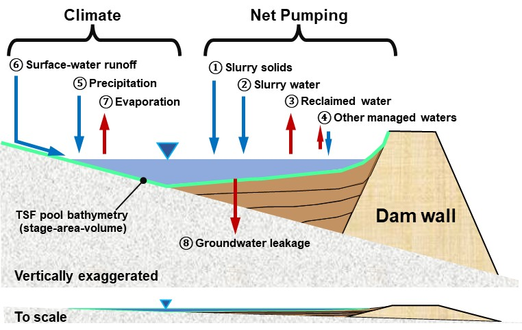
Tailings-Storage Facility Iterative Simulation Model or TSFISM is an Excel workbook that simulates the water balance and accumulation of tailings in a tailings-storage facility (TSF). Tailings are introduced into a TSF pool as a slurry comprised of slurry solids ① and slurry water ② (Figure 1). Pool stage usually is managed by pumping reclaimed water ③ from the TSF pool. Other managed waters ④, such as seepage to drains, also can be added or removed from a TSF pool. Slurry solids, slurry water, reclaimed water, and other process flows are managed actively and collectively analyzed as net pumping (Figure 1). Water balance of a TSF pool also is affected by local climate, where precipitation ⑤ and surface-water runoff from tailings beach ⑥ add water and evaporation ⑦ removes water (Figure 1). Flow rates of these three climatic terms depend on the surface area, which changes as tailings accumulate. Pool stage and bathymetry change as tailings accumulate and surface area changes in response to these operational changes (Jackson, et.al., 2026). Water also can seep from unlined facilities as uncaptured groundwater leakage ⑧ (Figure 1).
Water-Balance Data
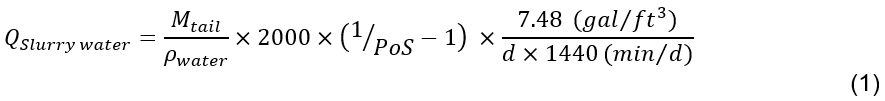
Volumes of slurry solids are estimated from production tailings (Figure 2). Slurry solid flow rates equal tailings production rates divided by specific gravity. These flow rates are reasonably certain because specific gravity of tailings typically average 2.65 with a limited range of specific gravities between 2.5 and 3.0 for gold and copper tailings (Vermeulen, 2001).
Volumes of slurry water are reported as percent of solids (PoS) and are more uncertain than volumes of slurry solids (Figure 2). Volume of slurry water in gallons per minute (gpm) is,
where,
Mtail is mass rate of tailings in short tons per month (M/T);
ρwater is density of water, 62.4 lbs/ft³ (M/L³);
PoS is percent of solids, denoted as a fraction; and
d is days (T) in month.
Estimated slurry water flow rates are disproportionally sensitive to PoS estimates. For example, slurry water volumes increase by 70 percent if PoS changes from 0.3 to 0.2 and decrease by 35 percent if PoS changes from 0.3 to 0.4 (Figure 2). Volumetric flow rate is illustrated with imperial units, but TSFISM also can be report volumetric flow rates in metric units.
Net pumping collectively is all managed water that is pumped from a TSF pool or returned to a TSF pool. Net pumping principally is reclaimed slurry water but also can include other discrete components, such as seepage to drains, which typically comprise less than a few percent of monthly reclaimed water volumes.
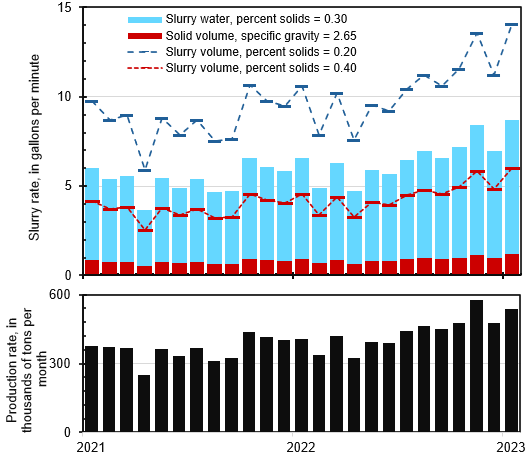
Slurry solids, slurry water, and reclaimed water are tracked in the water-balance model as net pumping (Figure 3). Net pumping is tracked because the water-balance model principally is affected by the combined flow of slurry and reclaimed water, not the individual components from plant data (Figure 1).
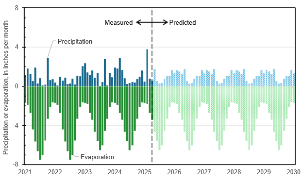
Climate components of the water balance of a TSF pool principally are defined by monthly measurements of precipitation and evaporation (Figure 4). Precipitation and evaporation typically are predicted by averaging and projecting long-term monthly averages. Alternatively, predicted precipitation and evaporation can be estimated with external models, where results supplant the projected long-term monthly averages.
Surface-water runoff to a TSF pool is estimated from time series of specified precipitation and catchment characteristics. Catchments are defined by area, runoff percentage, and threshold precipitation. These characteristics can change during the life of a TSF and, accordingly, are defined as time series. Surface-water runoff is simulated as available precipitation (L) times runoff percentage times catchment area minus pool area (L²). Available precipitation is specified precipitation minus threshold precipitation and is limited to 0 if threshold precipitation exceeds specified precipitation.
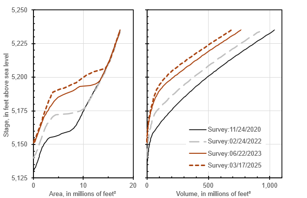
Changes in TSF pool geometry are measured with repeated bathymetric surveys that are summarized as stage-area-volume (SAV) relations (Figure 5). Accumulation of sediment and raising of pool elevation are monitored by increasing elevations of the pool bottom. Climate components of the TSF pool water budget are estimable because pool surface area is a function of stage. Sedimentation volumes in the TSF pool are measured by differencing volumes between repeated bathymetric surveys (Figure 5).
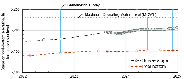
Pool stage is the principal measure of water budget and operability of a TSF (Figure 6). Pool stage directly measures proximity of the water surface to the Maximum Operating Water Level (MOWL) and indirectly measures changes in sedimentation and free-water volumes. These indirect estimates use measured pool stages to interpret sedimentation and free-water volumes from repeated bathymetric surveys (Figure 5).
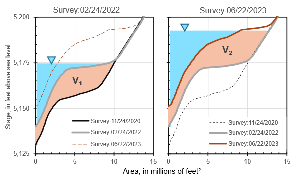
Sedimentation volume in the TSF pool is estimated each time a new bathymetric survey is measured. Sedimentation volume is the difference between volumes from the previous and new SAVs. These volumes are interpolated from the new surveyed pool stage and volume differences between the new and previous bathymetric surveys (Figure 7). For example, bathymetry was measured on 06/22/2023 when pool stage was 5,191.9 ft. Pool volume from the 06/22/2023 SAV was 119 million ft³ and equaled the volume of free-water because negligible sedimentation was assumed to occur during the bathymetric survey and above the pool stage. Pool volume would have equaled 272 million ft³ from the 02/24/2022 SAV for the same stage of 5,191.9 ft. The difference between these two volumes, V₂, equaled a sedimentation volume of 153 million ft³ that was deposited during the 483 days between bathymetric surveys (Figure 7).
Free-water volume in a TSF equals pool volume from the most recent bathymetric survey minus sedimentation volume since the most recent bathymetric survey. Free-water volume is best estimated immediately after a bathymetric survey when the volume from the SAV equals free-water volume. This interpretation reasonably assumes negligible sedimentation has occurred during the bathymetric survey.
Sedimentation volume is distributed proportionally to cumulative tailings production between bathymetric surveys (Figure 8). For example, pool stage was 5,188.0 ft on 03/31/2023 as interpolated between surveyed pool stages. Cumulative tails production totaled 11.68 million tons or 95 percent of tails production between the 02/24/2022 and 06/22/2023 bathymetric surveys. Cumulative sedimentation volume since the 02/24/2022 bathymetric survey was estimated as 145 million ft³ on 03/31/2023 or 95 percent of 153 million ft³ deposited between bathymetric surveys (Figure 8).
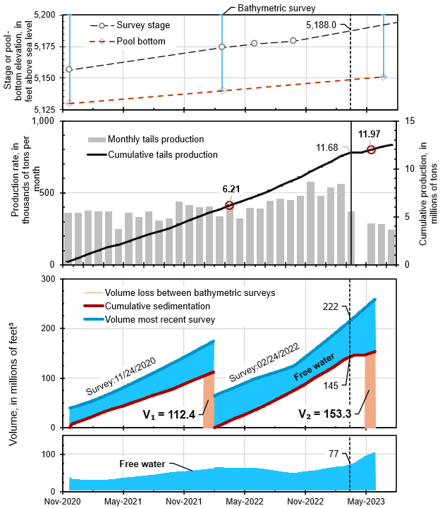
Free-water volume can be estimated continuously with temporally distributed sedimentation volumes (Figure 8). For example, free-water volume was 77 million ft³ on 03/31/2023. This was the difference between 222 million ft³ from the 02/24/2022 bathymetric survey minus 145 million ft³ of cumulative sedimentation (Figure 8).
Water-Balance Model
TSF-pool stage is simulated with a water balance approach that solves iteratively for change in pool volume and stage at the end of a time step (Figure 9). This approach is similar to water-balance models of pit lakes (Fontaine and others, 2003; Halford, 2025). Change in pool volume, ΔV, during a time step is,

where,
Δt is the time-step duration, [T];
Q is net pumping that sums rates of slurry addition (solids and water), reclaimed water subtraction, and other mine-related components, [L³/T];
QGW is the groundwater-leakage rate, computed using Amean [L³/T];
Amean is the pool area from averaging pool areas at the beginning and end of a time step [L²],
P is effective precipitation rate, where contributions from snow are tallied when snow melts rather than when snow accumulates, [L/T];
E is evaporation rate, in [L/T];
Pcatch-thresh,i is threshold precipitation rate of the ith catchment area at which runoff occurs, in [L/T];
ROcatch,i is precipitation runoff efficiency of the ith catchment, dimensionless;
Acatch,i is surface area of the ith catchment, [L²];
Pbeach is threshold precipitation rate of the beach at which runoff occurs, in [L/T];
RObeach is precipitation runoff efficiency of the beach, dimensionless; and
Abeach is surface area of the beach, [L²];
TSFISM sums all time-series of mine-related inflows and outflows to compute net pumping. The user specifies time series of tailings-production rates [M/T], percent solids, and specific gravity for the computation of slurry water and slurry solids. Reclaim water and other managed flows to and from the TSF also are user-defined as separate time series. Precipitation (P), open-water evaporation (E), runoff coefficients (RO), and catchment areas (A) also are user-specified as time series. The measurement frequency of these user-defined times series can differ from the time-step frequency simulated by TSFISM.
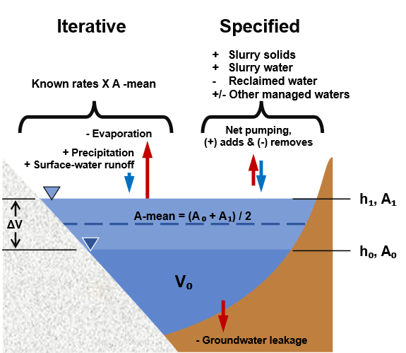
Groundwater leakage (GW) can be simulated with either hydraulic conductivity (L/T) or hydraulic conductance (1/T). Hydraulic conductivity is specified if sediments in the TSF are assumed to control leakage and GW is hydraulic conductivity (L/T) times a unit gradient (L/L). Hydraulic conductance is specified if pool-bottom sediments in the TSF are assumed to control leakage and GW is hydraulic conductance (1/T) times pool depth (L). Lined ponds with no groundwater leakage are simulated by specifying either hydraulic conductivity or hydraulic conductance as zero.
Changes during a time step are solved by initially assuming no change in pool stage so initial and final surface areas are the same during the first iteration. Surface area of the pool affects estimated precipitation, evaporation, groundwater leakage, and surface-water runoff during a time step. Change in pool volume, ΔV, is solved with equation (2) and added to the existing pool volume, V₀ (Figure 9). Pool stage at the end of a time step, h₁, is interpolated from the user-defined SAV relation with the new volume, V₀+ΔV. A revised pool area at the end of the time step, A₁, is interpolated from the SAV with the new pool stage h₁. This revises Amean, which changes the climatic stresses in equation (2) and revises estimates of ΔV and h₁. This process is repeated until simulated pool stage converges on a single value at the end of the time step (Figure 10).
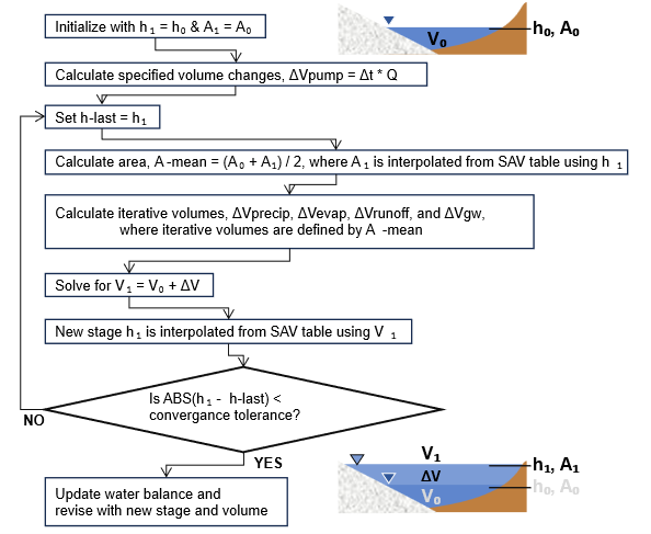
The water balance is solved differently if TSF pool goes dry, which occurs when ΔV is negative, and the magnitude exceeds V₀ (Figure 10). ΔV initially is reduced by curtailing groundwater leakage (GW), but curtailment cannot exceed magnitude of groundwater leakage (GW). Magnitude of ΔV is reduced to equal V₀ by curtailing net pumping. Specified and simulated net pumping can differ when simulated TSF pool goes dry (Jackson, et.al., 2026).
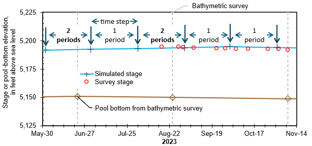
Stage and volume changes in a time step are simulated with two periods when a time step straddles a bathymetric survey (Figure 11). The first period simulates stage and volume change from the beginning of the time step to the bathymetric survey using the previous SAV. The second period simulates change from the bathymetric survey to the end of the time step using the new SAV. Simulated sedimentation volume is computed at the bathymetric survey by differencing volumes from previous and new SAVs. This is the same method for estimating surveyed free-water volumes except sedimentation volumes are interpreted with simulated stages rather than surveyed pool stages (Figure 7).
Free-water volumes are simulated continuously by the TSFISM model with simulated stages. This is the same approach for interpreting free-water volumes from surveyed stages except with simulated stages instead (Figure 8). Simulated sedimentation volume is distributed proportionally to cumulative tailings production between bathymetric surveys. Simulated free-water volume equals simulated pool volume minus simulated sedimentation volume since the most recent bathymetric survey (Figure 8).
Predicting TSF Operations
Predicting future TSF operations requires predicted rates of all water-balance inputs. Tailings production, reclaimed water, other managed waters, precipitation, evaporation, and surface-water runoff are readily forecast from operational plans and climate data. Changes in TSF pool geometry as measured with bathymetric surveys are more difficult to predict without additional analysis.
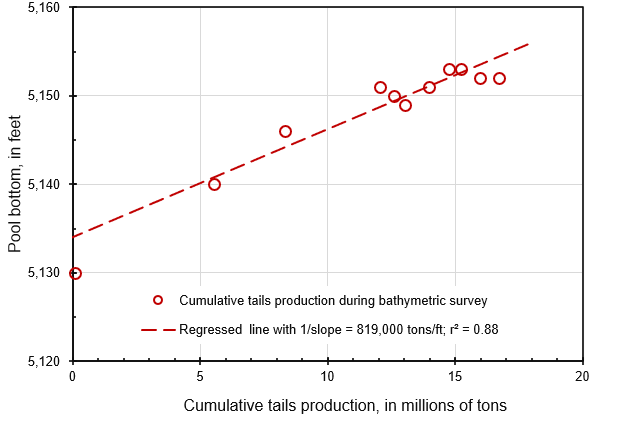
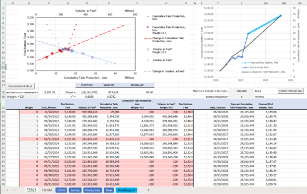
Measured pool-bottom elevations are correlated with cumulative tails production. Future pool-bottom elevations can be predicted from a regression between pool-bottom elevation and cumulative tails production that are tabulated for each bathymetric survey. For example, pool-bottom elevation increases 1 ft with each additional 819,000 tons of tailings (Figure 12), so adding 4.1 million tons of tails would be expected to raise the TSF pool 5.0 ft. A one-dimensional correlation between elevation and cumulative tails production works because surface area of a TSF changes minimally relative to vertical changes in a TSF (Figure 1; see “To scale”).
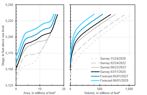
Future bathymetry can be predicted by assuming historical deposition plans are representative and the pool is simply elevated as tailings are added to a TSF (Figure 13). Future SAV relations remain the same as the SAV from the last bathymetric survey, except stages are elevated. Pool-bottom elevations increase proportionally to forecasted tailings production. For example, an additional 6.8 and 14.3 million tons of tails were forecasted to be added by May 2027 and June 2029, respectively, after March 2025. This raised the forecasted SAV by 8.3 and 17.4 ft since the last bathymetric survey measured March 17, 2025 (Figure 13).
Future deposition plans can change from historical plans and alternative methods of estimating future bathymetries are needed. Future SAV relations can be estimated with other methods and added to existing series of surveyed SAV relations. Surveyed and externally predicted SAV relations are differentiated so that only measured pool-bottom elevations are correlated with cumulative tails production (Figure 12).
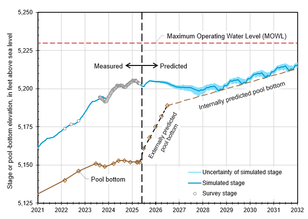
Both externally and internally predicted SAV relations can be used in a single simulation (Jackson, et.al., 2026). For example, surveyed, externally predicted, and internally predicted pool bottoms create a continuous pool-bottom elevation (Figure 14). Pool-bottom elevations are surveyed during the measured period. Externally predicted pool bottoms rise steeply in 2025 and 2026 and internally predicted SAV relations define the forecast pool bottom during the predicted period (Figure 14).
Uncertainty in predicted pool stages and free-water volumes principally reflects uncertainty in precipitation forecasts. Annual precipitation can vary markedly between years (Figure 4), which affects TSF pool stages. Uncertainty of annual precipitation is estimated with the log-Pearson Type III distribution, which is used prevalently for flood-frequency analysis (Interagency Advisory Committee on Water Data, 1982; Gotvald et al., 2012; England et al., 2018). Uncertainty of annual precipitation usually is reported as a range where 90 or 95 percent confidence exists that annual precipitation during a given year will be within the estimated range.
Uncertainty in predicted pool stages and free-water volumes are estimated with alternative models that simulate minimum and maximum precipitation within a specified confidence interval. Predicted precipitation in these alternative models scales long-term monthly averages by the ratio of predicted to average annual volumes of precipitation. This approach preserves seasonal variations in precipitation, which can be significant. For example, annual precipitation averaged 13.3 inches (Figure 4). The 95-percent confidence interval of annual precipitation from this distribution ranged between 7.4 and 19.5 inches. Predicted pool stages depart less than 3 ft from the average simulated pool stage, where annual precipitation ranges between 7.4 and 19.5 inches (Figure 14). A similar range of uncertainty also is reported for free-water volumes.
TSFISM workbook features
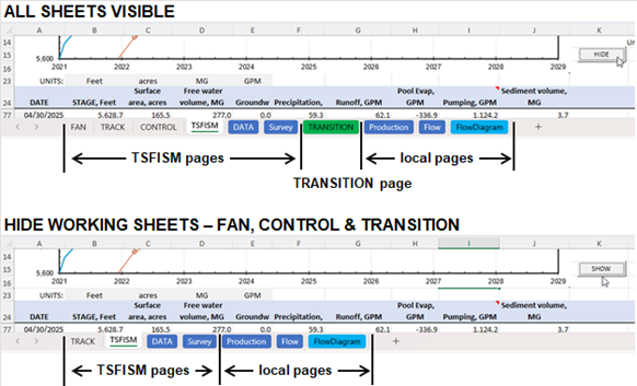
The workbook is composed of three groups of pages: TSFISM, local, and TRANSITION (Figure 15). TSFISM pages have a prescribed structure that should not be changed by the user. Local pages are structured and maintained by the user to record tailings production, percent solids, and flow rates of slurry, reclaimed water, and other managed waters (Figure 1). Local pages are supported in the TSFISM workbook to estimate net pumping (Q in eq. 2) and track cumulative tailings production for the water-balance model. TRANSITION is a single page for consistently passing data inputs from the local pages to the TSFISM water-balance model (Figure 15).
The TSFISM group consists of four visible pages, DATA, Survey, TRACK, and TSFISM, and two nominally hidden pages CONTROL and FAN (Figure 15). Time series of SAV relations from bathymetric surveys, maximum operating water levels, catchment characteristics, and precipitation, evaporation rates, and net pumping rates are specified on the DATA page. Surveyed stages are specified and interpreted pool areas, and free-water volumes are reported on the Survey page. Pool-bottom elevations and cumulative tailings production are reported and analyzed on the TRACK page. Simulated pool stages and free-water volumes are reported and analyzed on the TSFISM page. The hidden CONTROL page contains lookup tables, unit conversions, charting utilities, and water-balance model. The hidden FAN page is a template for reporting climatic uncertainty analyses. Both hidden pages should not be edited by users.
Water balance of the TSF pool principally is analyzed from the TSFISM page (Figure 16). Surveyed and simulated stages can be compared and differences minimized by adjusting hydraulic conductivity/vertical leakance on the TSFISM page or groundwater leakage or the time series of PoS in the local pages. Surveyed and simulated stages also can be compared to significant references such as the pool bottom and freeboard (MOWL) (Figure 16). Surveyed and simulated free-water volumes also can be compared while minimizing differences (Figure 17; B).
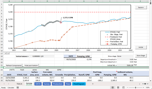
Surveyed and simulated free-water volumes are displayed on a separate chart from surveyed and simulated stages on the TSFISM page (Figure 17). A third chart also exists that displays flow rates for each water-balance component by time step (Figure 17; C). Display areas of these three charts are maximized by being stacked on top of one another so that only one chart is visible at a time (Figure 16). Chart visibility is changed by a spin button (cell A17) that charts up or down in the stack.
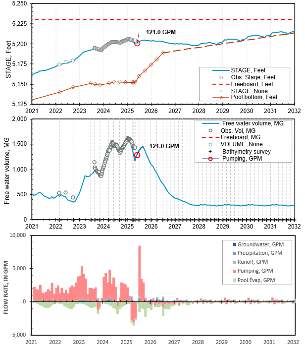
B.) surveyed and simulated free-water volumes, and C.) rates of flow components to and from TSF pool as reported by TSFISM workbook.
Measured pool-bottom elevations and cumulative tails production are synthesized on the TRACK page so that future pool-bottom elevations can be predicted (Figure 18). Macros reduce SAV relations from bathymetric surveys on the DATA page and return cumulative tails production from monthly tails production on the TRANSITION page. Time series of SAV relations are reduced to pool-bottom elevations and free-water volumes relative to a common maximum stage.
Regression between measured pool-bottom elevations and cumulative tails production is controlled by weighting observations (Figure 18). This allows pool-bottom elevations from outlying bathymetric surveys and externally forecasted SAV relations to be excluded. Regressing measured pool-bottom elevations against consistent free-water volumes allows for tailings density to be estimated. This provides an additional test of the plausibility of forecasted rate of pool-bottom elevation rise.
Future SAV relations are elevated with an empirically estimated rate of pool rise per mass of forecasted tailings production. These internally estimated SAV relations are appended to existing SAV relations from bathymetric surveys and external forecasts on the DATA page. These internally predicted SAV relations are differentiated from surveyed and externally predicted SAV relations.
Macros were developed in Microsoft Excel® 365 and are not backward compatible to earlier versions of Excel. This is because user-defined functions use previously unavailable SPILL functionality to return two-dimensional arrays.
VBA macros & Trust Center
More macro functions default to being disabled through either Microsoft updates or IT departments engaging in their natural function. Please check your Trust Center settings.
Download
The file TSFISM.v12.zip contains,
- TSFISM.v12.xlsm – Workbook with TSFISM model;
- FullRainfall-StormAnalysis.xlsx – Example of annual precipitation analysis to estimate range of predicted pool stages and volumes in a tailings-storage facility; and
- TSFISM-EXPLAIN.v12.pdf – Explanatory document.
Revisions
March 31, 2026—Revisions through version 10 comprise initial release.
April 17, 2026—Revisions in version 11 include the following. Corrected errors in function vShiftLastRESID that failed where simulation period less than SAV frequency. Corrected error in catchment-runoff table, where only last row was used instead of all rows for a given time. Cleaned excess cell styles that were introduced accidentally to the TSFISM example/template.
May 18, 2026— Revisions in version 12 include the following. Corrected conversion errors for freeboard and pool elevations. Revised suggested citation to published article.
Suggested Citation
Jackson, T.R., Halford, K.J. & Zhan, G., 2026, Tailings Storage Facility Iterative Simulation Model (TSFISM): A Dynamic Simulator, Mine Water and the Environment, https://doi.org/10.1007/s10230-026-01124-w
or
Halford, Keith, 2026, TSFISM–An Excel workbook for simulating the water balance of a tailings-storage facility, version 12, Halford Hydrology LLC web page, accessed May 2026, at https://halfordhydrology.com/tsfism/
References
England, J.F., Jr., Cohn, T.A., Faber, B.A., Stedinger, J.R., Thomas, W.O., Jr., Veilleux, A.G., Kiang, J.E., and Mason, R.R., Jr., 2018, Guidelines for determining flood flow frequency — Bulletin 17C (ver. 1.1, May 2019): U.S. Geological Survey Techniques and Methods, book 4, chap. B5, 148 p., https://doi.org/10.3133/tm4B5
Fontaine, R.C., A. Davis, and G.G. Fennemore, 2003, The Comprehensive Realistic Yearly Pit Transient Infilling Code (CRYPTIC): A Novel Pit Lake Analytical Solution, Mine Water and the Environment v.22 pgs. 187–193 https://doi.org/10.1007/s10230-003-0021-z
Gotvald, A.J., Barth, N.A., Veilleux, A.G., and Parrett, C., 2012, Methods for determining magnitude and frequency of floods in California, based on data through water year 2006: U.S. Geological Survey Scientific Investigations Report 2012–5113, 38 p., 1 pl., https://doi.org/10.3133/sir20125113
Halford, K., 2025, Analytical_PLISM–An Excel workbook for simulating water balance of a pit lake, version 5, Halford Hydrology LLC web page, accessed March 2025, at https://halfordhydrology.com/plism/
Interagency Advisory Committee on Water Data, 1982, Guidelines for determining flood flow frequency: Hydrology Subcommittee Bulletin 17B, 28 p., 14 app., 1 pl. https://water.usgs.gov/osw/bulletin17b/dl_flow.pdf
Jackson, T.R., Halford, K.J. & Zhan, G., 2026, Tailings Storage Facility Iterative Simulation Model (TSFISM): A Dynamic Simulator, Mine Water and the Environment, https://doi.org/10.1007/s10230-026-01124-w
Vermeulen, N.J., 2001, The Composition and State of Gold Tailings: University of Pretoria Doctoral Thesis, 441 p. http://hdl.handle.net/2263/23079